Hi, my name is Henrique and I am an undergraduate student in Chemistry doing some theoretical research about Fe(II) in water as a requirement to finish my graduation.
I’ve been using ORCA to perform some calculations and to generate UV-vis spectra of [Fe(OH2)6]2+ and [Fe(OH2)6]3+.
The result for [Fe(OH2)6]2+ is pretty much what I was expecting, but for [Fe(OH2)6]3+ it seems a little weird to me:
Since the d5 Iron(III) have only spin forbidden transitions, I wasn’t expecting it to have more intense Abs than iron(II) (see attachment).
I wasn’t able to put my hands in any [Fe(OH2)6]3+ UV-vis spectra to compare with my results and I’d like to read some opinions about this issue:
· Is there something wrong with my input?
·
Does
this spectra (attached) look weird to you or there is a good explanation for
Fe(III) to
have a more intense Abs than 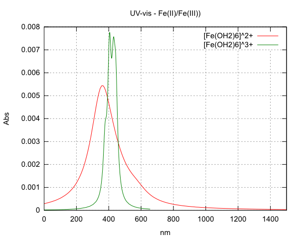 Fe(II)?
Thank you for any advice and I am very sorry for my poor English.
--------------------------------------------INPUT-----------------------------------------------------------------------------
# ================================================================
# Orca input file made in Gabedit
# ================================================================
! RI Opt TightSCF BP86
! PrintBasis Def2-TZVP Def2-TZVP/C
%tddft
nroots 8 # the number of excited states to be calculated.
maxdim 30 # the maximum dimension of the expansion space in the Davidson procedure.
# dcorr n
# n=1-4. The meaning of the four algorithms
# algorithm 1 Is perhaps the best for small systems. May use a
# lot of disk space
# algorithm 2 Stores less integrals
# algorithm 3 Is good if the system is large and only a few
# states are to be made. Safes disk and main memory.
# algorithm 4 Uses only transformed RI integrals. May be the
# fastest for large systems and a larger number of states
# TammDanCoff true Tamm-Dancoff approximation for non-hybride
# Triplets true : do triplets states
# EWin -3,100 (orbital energy window in Eh)
# Etol 1e-3 the required convergence of the energies of the excited states (in Eh)
# Rtol 1e-5 required convergence on the norm of the residual vectors.
# essential for metal edges. For ligand edges, the contributions are much smaller.
end #tddft
%output
print[p_mos] 1
end #output
%geom
MaxIter 500
end
%scf
MaxIter 500
end
* xyz 3 6
H -2.424829 -0.275250 0.279753
O -1.892119 -0.263000 -0.507137
H -2.224729 0.402440 -1.098897
H -0.919139 -0.831680 2.037573
H -0.592969 -2.430170 -0.174157
H -0.753899 0.722610 2.113113
O -0.385119 -0.088000 1.781863
O 0.240881 -1.977000 -0.121137
H -1.040679 2.169210 0.255553
H 0.720741 -2.264950 0.647723
Fe 0.008881 -0.041000 -0.127137
H -0.382459 0.048440 -2.580397
O -0.216119 1.897000 -0.131137
O 0.396881 -0.003000 -2.039137
H -0.141579 2.272920 -1.000737
H 1.024291 0.667680 -2.284267
O 1.909881 0.185000 0.245863
H 2.443031 -0.318650 -0.359427
H 2.165121 1.100290 0.221463
*
Química Industrial - UFRRJ
Centro de Processamento de Dados - PMP